Plotting with Marsilea

Marsilea is a visualization library that allows user to create composable visualization in a declarative way.

You can use it to create many scanpy plots with easy customization.

Let’s first load the PBMC datdaset

import numpy as np
import scanpy as sc

pbmc = sc.datasets.pbmc3k_processed().raw.to_adata()
pbmc

AnnData object with n_obs × n_vars = 2638 × 13714
    obs: 'n_genes', 'percent_mito', 'n_counts', 'louvain'
    var: 'n_cells'
    uns: 'draw_graph', 'louvain', 'louvain_colors', 'neighbors', 'pca', 'rank_genes_groups'
    obsm: 'X_pca', 'X_tsne', 'X_umap', 'X_draw_graph_fr'
    obsp: 'distances', 'connectivities'

Define the cells and markers that we want to draw

cell_markers = {
    "CD4 T cells": ["IL7R"],
    "CD14+ Monocytes": ["CD14", "LYZ"],
    "B cells": ["MS4A1"],
    "CD8 T cells": ["CD8A"],
    "NK cells": ["GNLY", "NKG7"],
    "FCGR3A+ Monocytes": ["FCGR3A", "MS4A7"],
    "Dendritic cells": ["FCER1A", "CST3"],
    "Megakaryocytes": ["PPBP"],
}

cells, markers = [], []
for c, ms in cell_markers.items():
    cells += [c] * len(ms)
    markers += ms

uni_cells = list(cell_markers.keys())
cell_colors = [
    "#568564",
    "#FFF3A7",
    "#F72464",
    "#005585",
    "#9876DE",
    "#405559",
    "#58DADA",
    "#F85959",
]
cmapper = dict(zip(uni_cells, cell_colors))

Import Marsilea

import marsilea as ma
import marsilea.plotter as mp

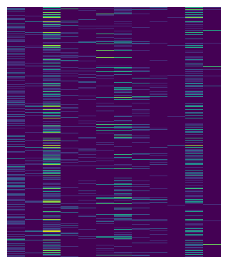
Heatmap

Here is the minimum example to create a heatmap with Marsilea, it does nothing besides create a heatmap. You can adjust the main plot size by setting height and width, the unit is inches.

We will start adding components to this main plot step by step.

exp = pbmc[:, markers].X.toarray()

m = ma.Heatmap(exp, cmap="viridis", height=3.5, width=3)
m.render()

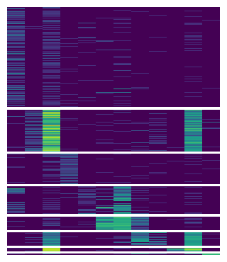
To replicate the scanpy heatmap, we can first divide the heatmap by cell types.

The hsplit stands for horizontal split, labels is used to label the row, the order define the display order of each cell types from top to bottom.

m.hsplit(labels=pbmc.obs["louvain"], order=uni_cells)
m.render()

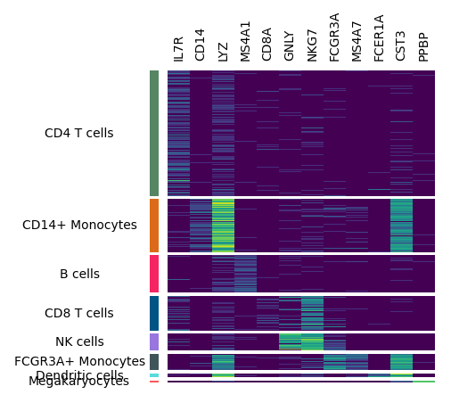
Now we can label each chunks with cell types and the columns with marker names.

You can use add_left or add_* to add a plotter to anyside of your main plot. In Marsilea, a plot instance is called plotter.

When you add a plotter, you can easily adjust its size and the padding between adjcent plot using size and pad.

# Create plotters
chunk = mp.Chunk(uni_cells, rotation=0, align="center")
colors = mp.Colors(list(pbmc.obs["louvain"]), palette=cmapper)
label_markers = mp.Labels(markers)

# Add to the heatmap
m.add_left(colors, size=0.1, pad=0.1)
m.add_left(chunk)
m.add_top(label_markers, pad=0.1)
m.render()

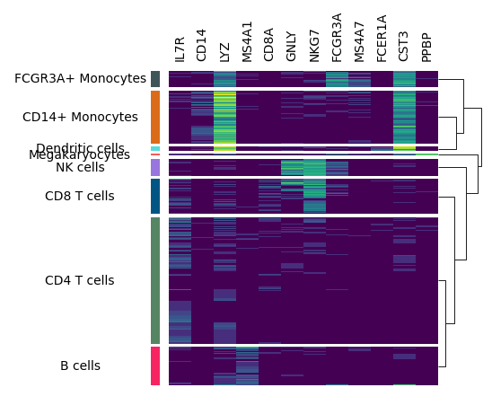
You may want to add dendrogram to display the similarity among cell types.

You can use add_dendrogram, we will add it to the right side, but you can also add it to the left side if you want.

m.add_dendrogram("right", add_base=False)
m.render()

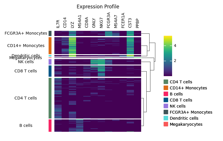
The legend is still mising, you can use add_legends to add all legends at once. Marsilea will automatically layout all the legends.

In the end, you can you add_title to add a title.

m.add_legends()
m.add_title("Expression Profile")
m.render()

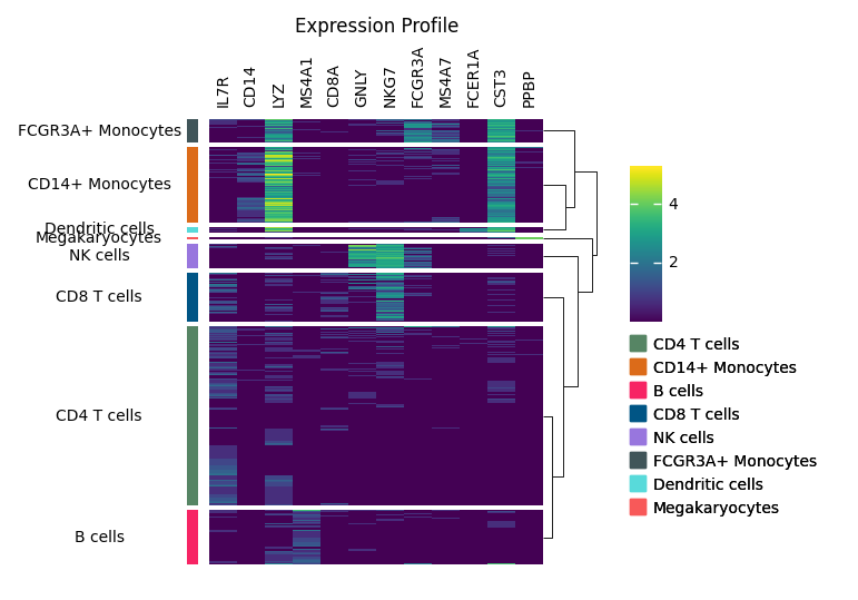
OK, let’s wrap up all the code in below. There are few things you should notice in Marsilea:

• Always call render() in the end to actually render the plot.

• The order of add_* operation decides the order of plotters. But vsplit and hsplit can be called anytime.

m = ma.Heatmap(exp, cmap="viridis", height=4, width=3)
m.hsplit(labels=pbmc.obs["louvain"], order=uni_cells)

m.add_left(
    mp.Colors(list(pbmc.obs["louvain"]), palette=cmapper),
    size=0.1,
    pad=0.1,
)
m.add_left(mp.Chunk(uni_cells, rotation=0, align="center"))
m.add_top(mp.Labels(markers), pad=0.1)
m.add_dendrogram("right", add_base=False)

m.add_legends()
m.add_title("Expression Profile")
m.render()

Now that we’ve covered some basics of Marsilea, we’ll see how it can be used to create custom plots similar to scanpy’s existing methods:

agg = sc.get.aggregate(pbmc[:, markers], by="louvain", func=["mean", "count_nonzero"])
agg.obs["cell_counts"] = pbmc.obs["louvain"].value_counts()
agg

AnnData object with n_obs × n_vars = 8 × 12
    obs: 'louvain', 'cell_counts'
    var: 'n_cells'
    layers: 'mean', 'count_nonzero'

exp = agg.layers["mean"]
count = agg.layers["count_nonzero"]
cell_counts = agg.obs["cell_counts"].to_numpy()

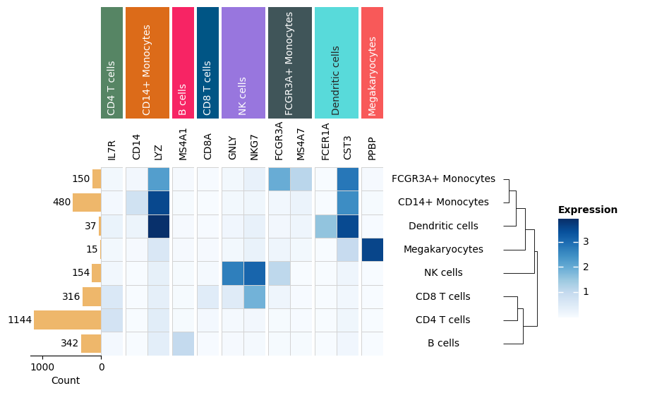
Matrixplot

h, w = exp.shape

m = ma.Heatmap(
    exp,
    height=h / 3,
    width=w / 3,
    cmap="Blues",
    linewidth=0.5,
    linecolor="lightgray",
    label="Expression",
)
m.add_right(mp.Labels(agg.obs["louvain"], align="center"), pad=0.1)
m.add_top(mp.Labels(markers), pad=0.1)
m.vsplit(labels=cells, order=uni_cells)
m.add_top(mp.Chunk(uni_cells, fill_colors=cell_colors, rotation=90))
m.add_left(mp.Numbers(cell_counts, color="#EEB76B", label="Count"))
m.add_dendrogram("right", pad=0.1)
m.add_legends()
m.render()

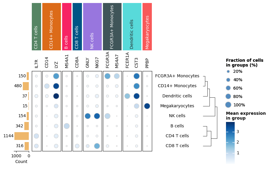
Dot plot

size = count / cell_counts[:, np.newaxis]
m = ma.SizedHeatmap(
    size=size,
    color=exp,
    cluster_data=size,
    height=h / 3,
    width=w / 3,
    edgecolor="lightgray",
    cmap="Blues",
    size_legend_kws=dict(
        colors="#538bbf",
        title="Fraction of cells\nin groups (%)",
        labels=["20%", "40%", "60%", "80%", "100%"],
        show_at=[0.2, 0.4, 0.6, 0.8, 1.0],
    ),
    color_legend_kws=dict(title="Mean expression\nin group"),
)

m.add_top(mp.Labels(markers), pad=0.1)
m.add_top(mp.Chunk(uni_cells, fill_colors=cell_colors, rotation=90))
m.vsplit(labels=cells, order=uni_cells)

m.add_right(mp.Labels(agg.obs["louvain"], align="center"), pad=0.1)
m.add_left(mp.Numbers(cell_counts, color="#EEB76B", label="Count"), size=0.5, pad=0.1)
m.add_dendrogram("right", pad=0.1)
m.add_legends()
m.render()

More information

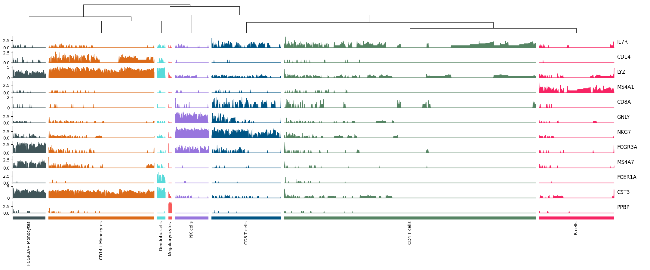
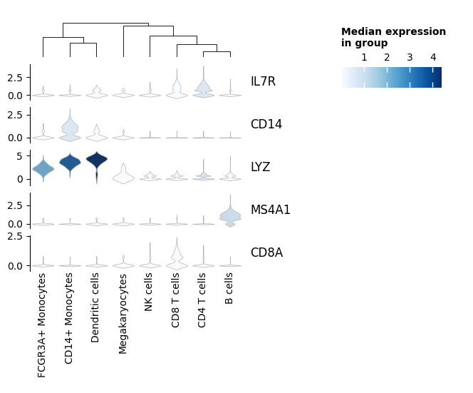
Futhrer plots, like tracksplot and stacked violin, are possible with Marsilea by creating new plotter. See Marsilea’s documention to learn how.

import session_info

session_info.show(dependencies=True)

Click to view session information

-----
anndata             0.10.6
marsilea            0.3.2
numpy               1.26.3
scanpy              1.10.0
session_info        1.0.0
-----

Click to view modules imported as dependencies

PIL                 10.2.0
asttokens           NA
colorama            0.4.6
comm                0.2.1
cycler              0.12.1
cython_runtime      NA
dateutil            2.8.2
debugpy             1.8.0
decorator           5.1.1
executing           2.0.1
h5py                3.10.0
ipykernel           6.29.1
jedi                0.19.1
joblib              1.3.2
kiwisolver          1.4.5
legacy_api_wrap     NA
legendkit           0.3.4
llvmlite            0.42.0
matplotlib          3.8.2
matplotlib_inline   0.1.6
mpl_toolkits        NA
natsort             8.4.0
numba               0.59.0
packaging           23.2
pandas              2.2.0
parso               0.8.3
patsy               0.5.6
pickleshare         0.7.5
platformdirs        4.2.0
prompt_toolkit      3.0.42
psutil              5.9.8
pure_eval           0.2.2
pydev_ipython       NA
pydevconsole        NA
pydevd              2.9.5
pydevd_file_utils   NA
pydevd_plugins      NA
pydevd_tracing      NA
pygments            2.17.2
pyparsing           3.1.1
pytz                2024.1
scipy               1.12.0
seaborn             0.13.2
six                 1.16.0
sklearn             1.4.0
stack_data          0.6.2
statsmodels         0.14.1
threadpoolctl       3.2.0
tornado             6.3.3
traitlets           5.14.1
typing_extensions   NA
vscode              NA
wcwidth             0.2.13
zmq                 25.1.2

-----
IPython             8.21.0
jupyter_client      8.6.0
jupyter_core        5.7.1
-----
Python 3.12.1 | packaged by conda-forge | (main, Dec 23 2023, 08:03:24) [GCC 12.3.0]
Linux-5.15.0-101-generic-x86_64-with-glibc2.35
-----
Session information updated at 2024-04-05 19:06